Quickstart

This guide provides a basic overview of UTDQuake and demonstrates how to access datasets, networks, events, and visualizations.

Warning

Make sure to use the latest stable version of UTDQuake.

You can follow this guide interactively in Colab:

Dataset Overview

To get started, import the package and load the dataset using the utdquake.Dataset class:

import utdquake as utdq

# dataset overview
dataset = utdq.Dataset(das=False) # set das=True to load DAS data
print(dataset)

# network level
network_data = dataset.networks
display(network_data)

In addition to network-level access, the dataset allows you to retrieve aggregated information across multiple networks. You can directly access events, stations, and picks using the following methods:

utdquake.Dataset.get_events() – retrieve event information across networks
utdquake.Dataset.get_stations() – retrieve station metadata
utdquake.Dataset.get_picks() – retrieve seismic phase picks

Network Data

Detailed information for a specific seismic network can be accessed through the utdquake.Network class:

# load network
network = dataset.get_network(name="tx")
display(network)

# events
events = network.events
display(events)

# stations
stations = network.stations
display(stations)

# picks
picks = network.picks
display(picks)

Event Bank

UTDQuake integrates an event bank. Check ObsPlus EventBank for more details.

# get event bank
ebank = network.bank #

# Example: Filter by event_id
ev_ids = events["event_id"].iloc[:5].tolist()
cat = ebank.get_events(event_id=ev_ids)
print(cat)

# Example 2: Other filter (check obsplus.EventBank for more details)
cat2 = ebank.get_events(minmagnitude=4.3)
print(cat2)

Catalogs to UTDQuake

UTDQuake provides convenient functions to convert catalogs to UTDQuake format.

Apply QC

import utdquake as utdq # Make sure we have the package imported to access the conversion functions
import logging # use logging to see the QC process in the console
logging.basicConfig(level=logging.DEBUG)

cat.apply_utdq_qc(debug=True, inplace=True)
print(cat)

Minimum QC criteria applied to events and picks.
Category	Parameter	Value
Event	Minimum associated phase count	4
Event	Minimum used phase count	4
Event	Minimum station count	3
Event	Maximum standard error	1.8
Pick	Minimum travel time	0
Pick	Minimum hypocentral distance	0
Pick	Minimum epicentral distance	0
Pick	Minimum S-P time difference (including `Sn-Pn` and `Sg-Pg`)	> 0

Convert to UTDQuake Format

import utdquake as utdq # Make sure we have the package imported to access the conversion functions
print("Events")
display(cat.utdq_events_to_df())
print("Picks")
display(cat.utdq_picks_to_df())

Events
time	latitude	longitude	depth	magnitude	event_id	…
2025-01-14 10:18:25	31.962	-102.990	8618.2	1.8	texnet2025aynz	…
2025-01-14 12:19:34	31.731	-104.092	6574.1	1.6	texnet2025aysb	…

Picks
network	station	phase	time	travel_time (s)	distance (deg)	…
2T	EF73	P	2025-01-30 03:26:40.660782	3.782	0.087	…
2T	EF61	P	2025-01-30 03:26:41.636254	4.757	0.138	…
TX	EF04	P	2025-01-30 03:26:41.924392	5.045	0.159	…

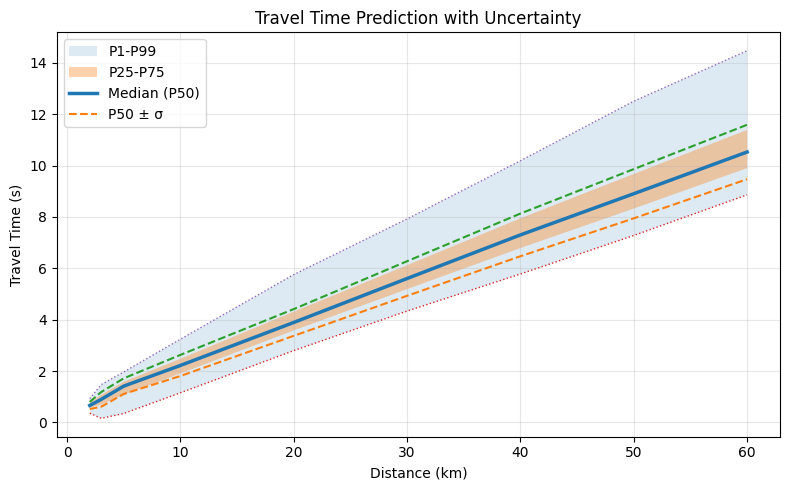
Travel Time Model

UTDQuake creates a travel time model for each network based on the information provided by the catalog.

tt = network.travel_time
predictions = tt.predict(phase="P", distance=[2,3,4,5,10,20,30,40,50,60]) #in km
display(predictions)

distance (km)	sigma (s)	p1 (s)	p25 (s)	p50 (s)	p75 (s)	p99 (s)
2	0.138	0.360	0.578	0.661	0.768	0.924
3	0.285	0.160	0.694	0.896	1.077	1.468
4	0.295	0.254	0.888	1.155	1.331	1.717
5	0.304	0.349	1.083	1.414	1.584	1.966
10	0.411	1.154	1.907	2.220	2.479	3.241

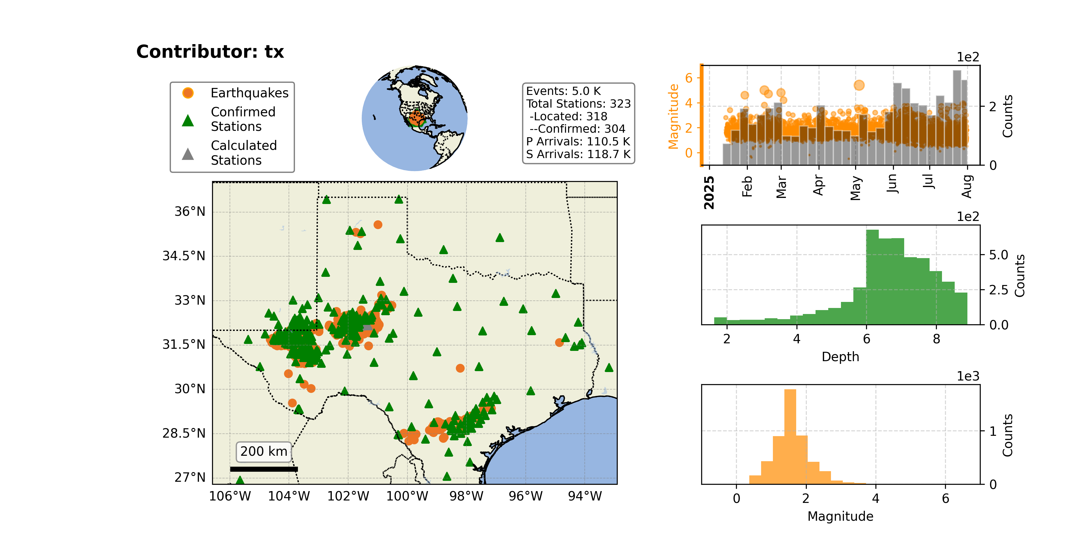
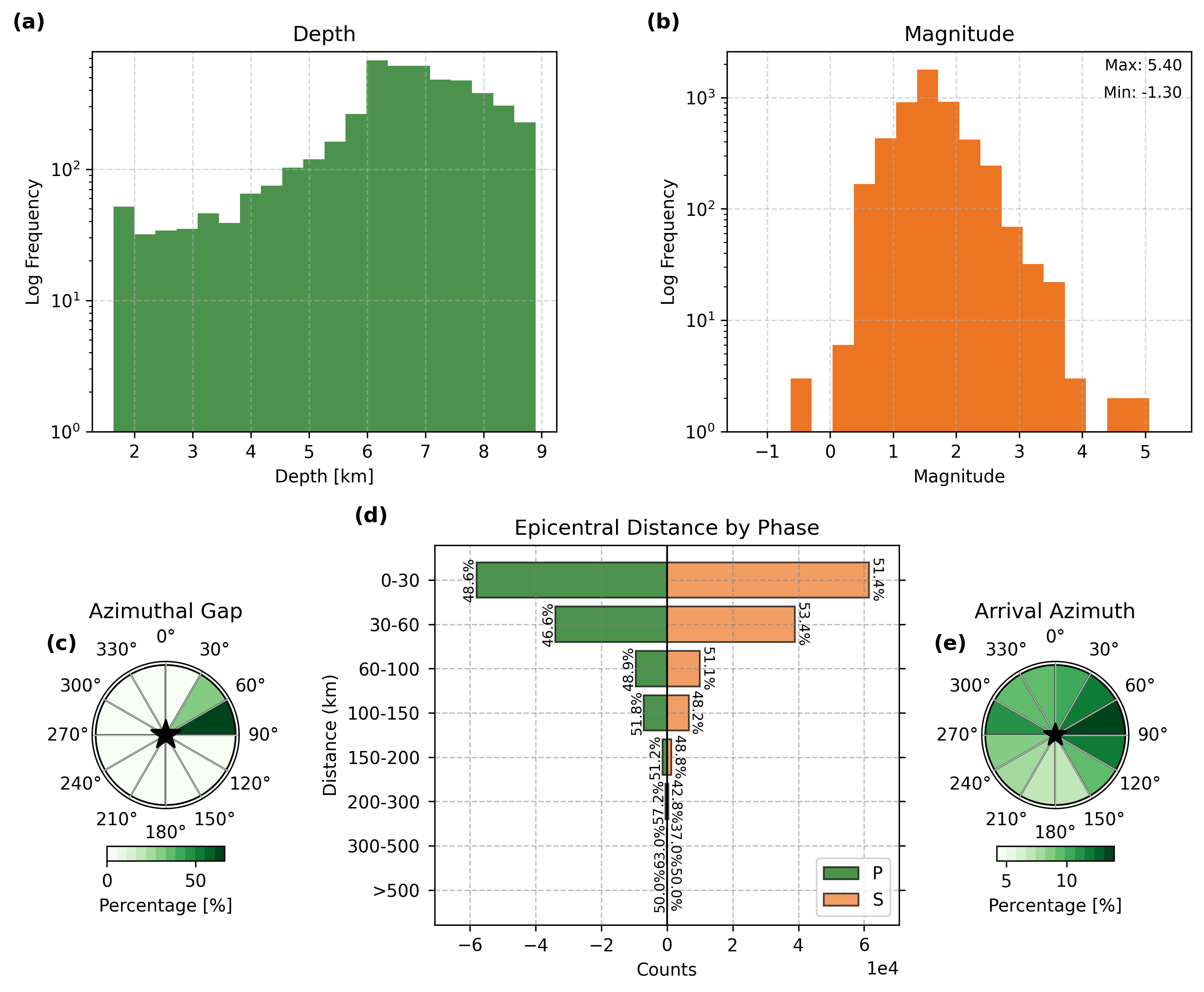
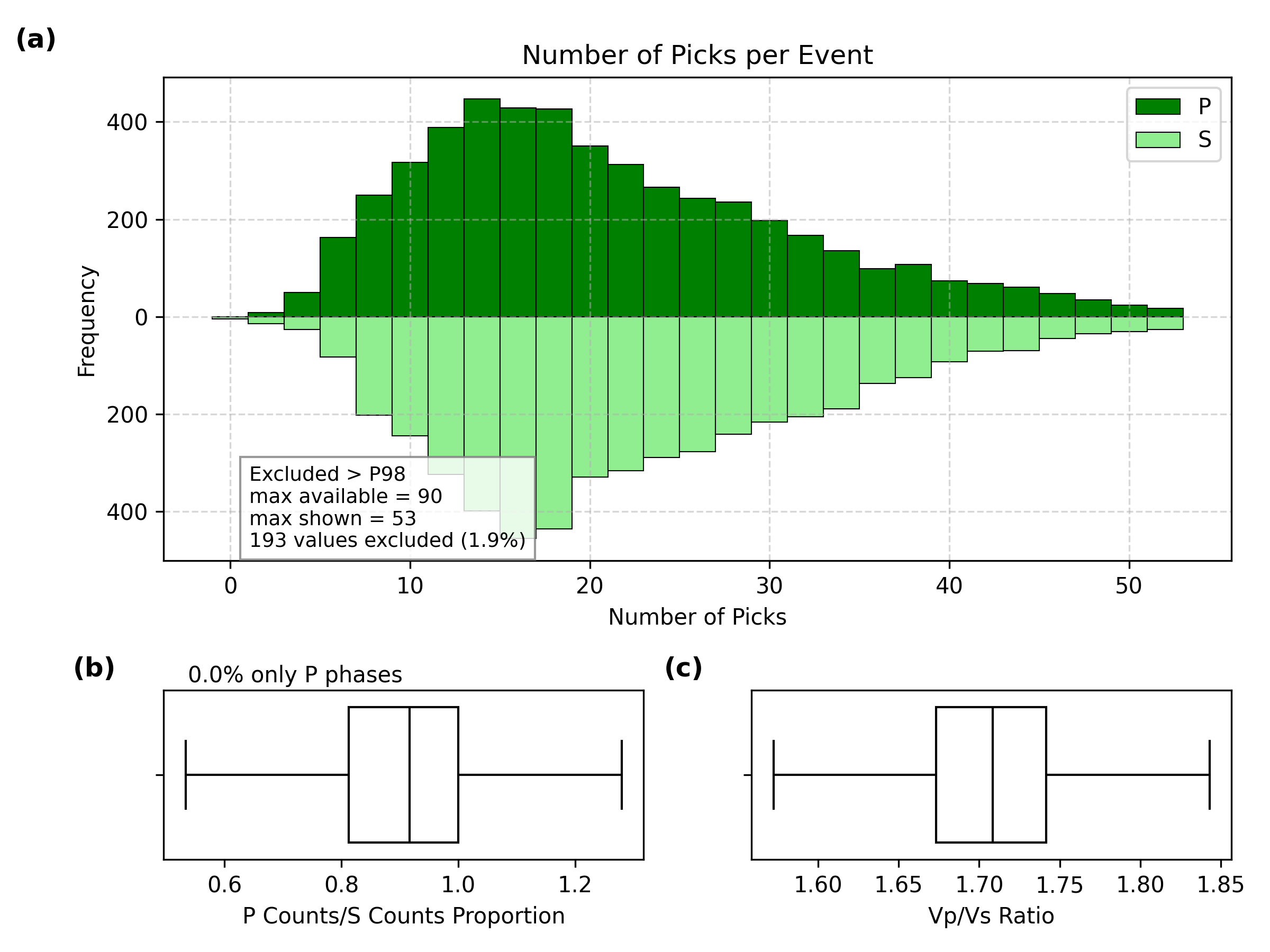
Visualization (Plots)

UTDQuake provides convenient plotting functions for quick data exploration. Check the utdquake.Network() plotting functions for more details and examples. Or also check the utdquake.utils.plot() module for more flexibility to create your own custom plots.

import utdquake as utdq

dataset = utdq.Dataset()
dataset.plot_overview(savepath="utdquake.png")

network = dataset.get_network(name="tx")

network.plot_overview(savepath="overview.png")
network.plot_stats(savepath="stats.png")
network.plot_pick_histograms(savepath="histograms.png")
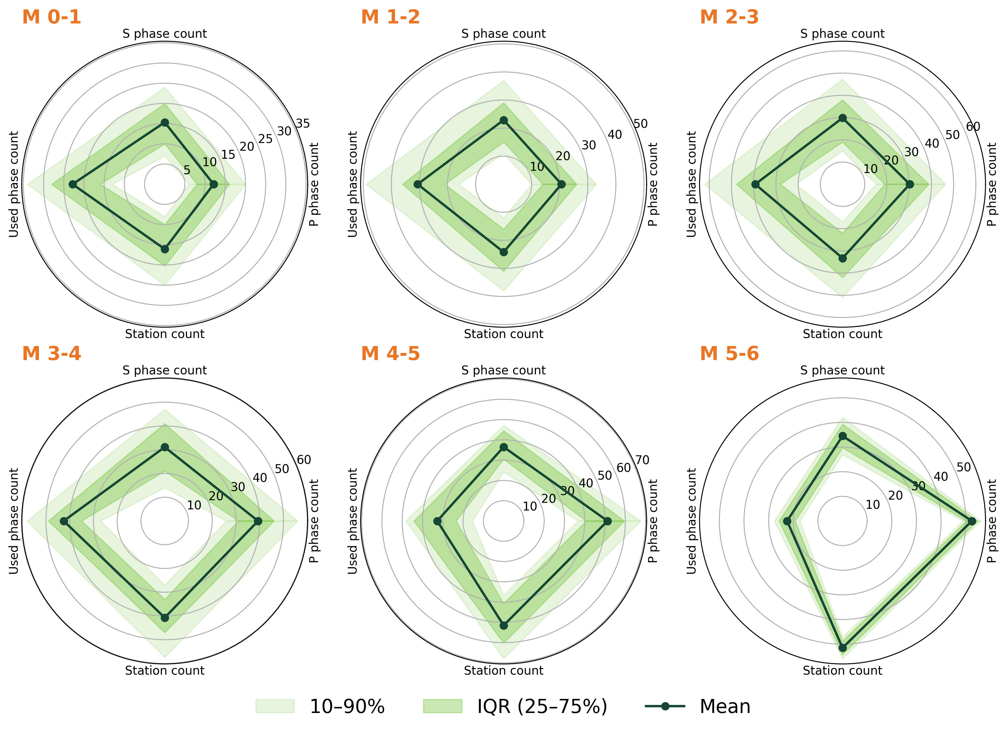
network.plot_phase_count_radar_by_magnitude(savepath="phase_count_radar.png")
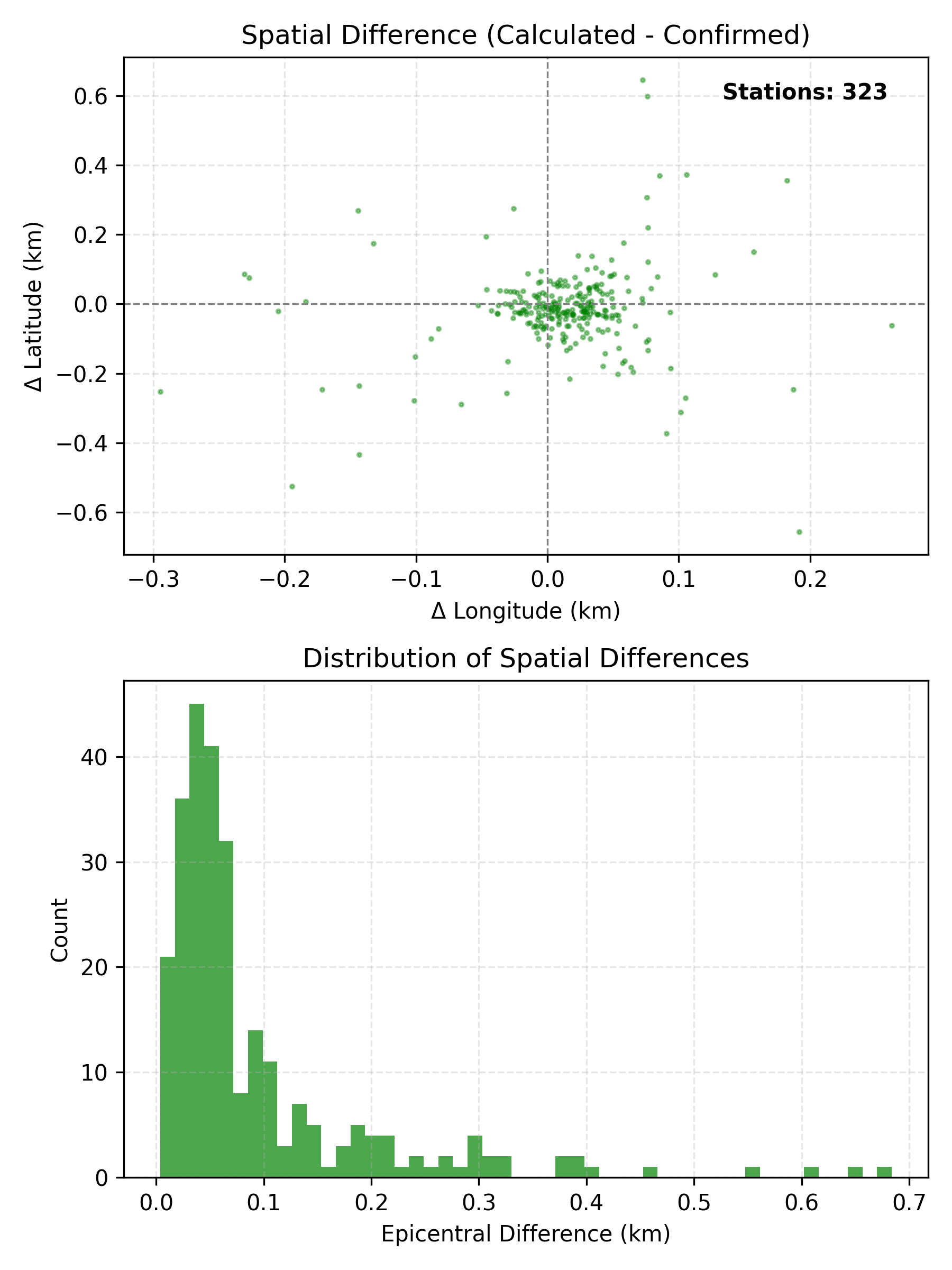
network.plot_station_location_uncertainty(savepath="station_location_uncertainty.png")
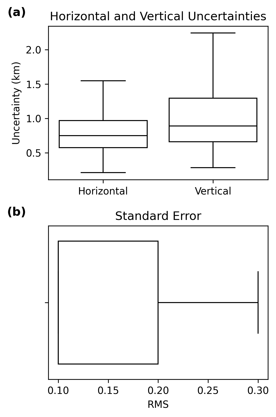
network.plot_uncertainty_boxplots(savepath="uncertainty_boxplots.png")
network.plot_travel_time_qc(savepath="plot_travel_time_qc.png")
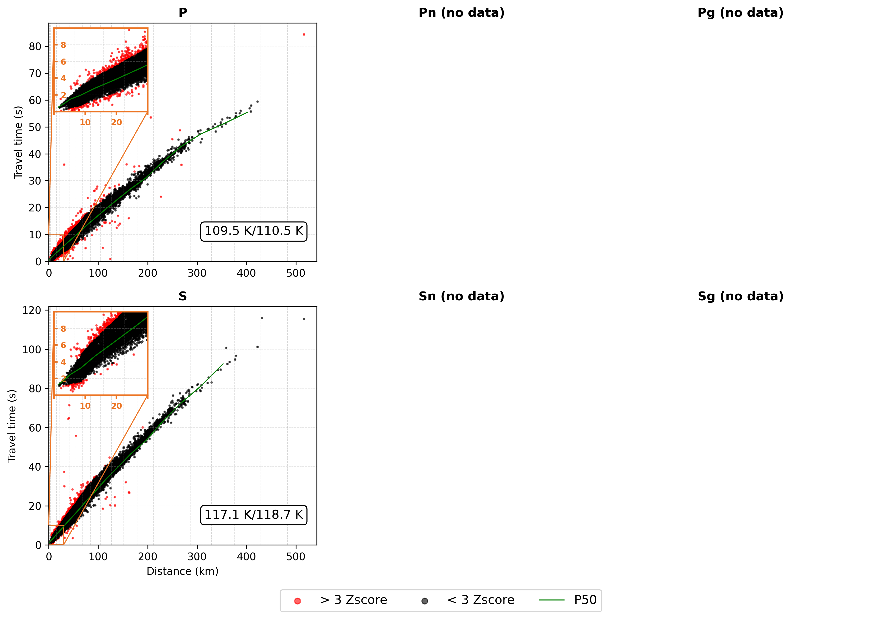
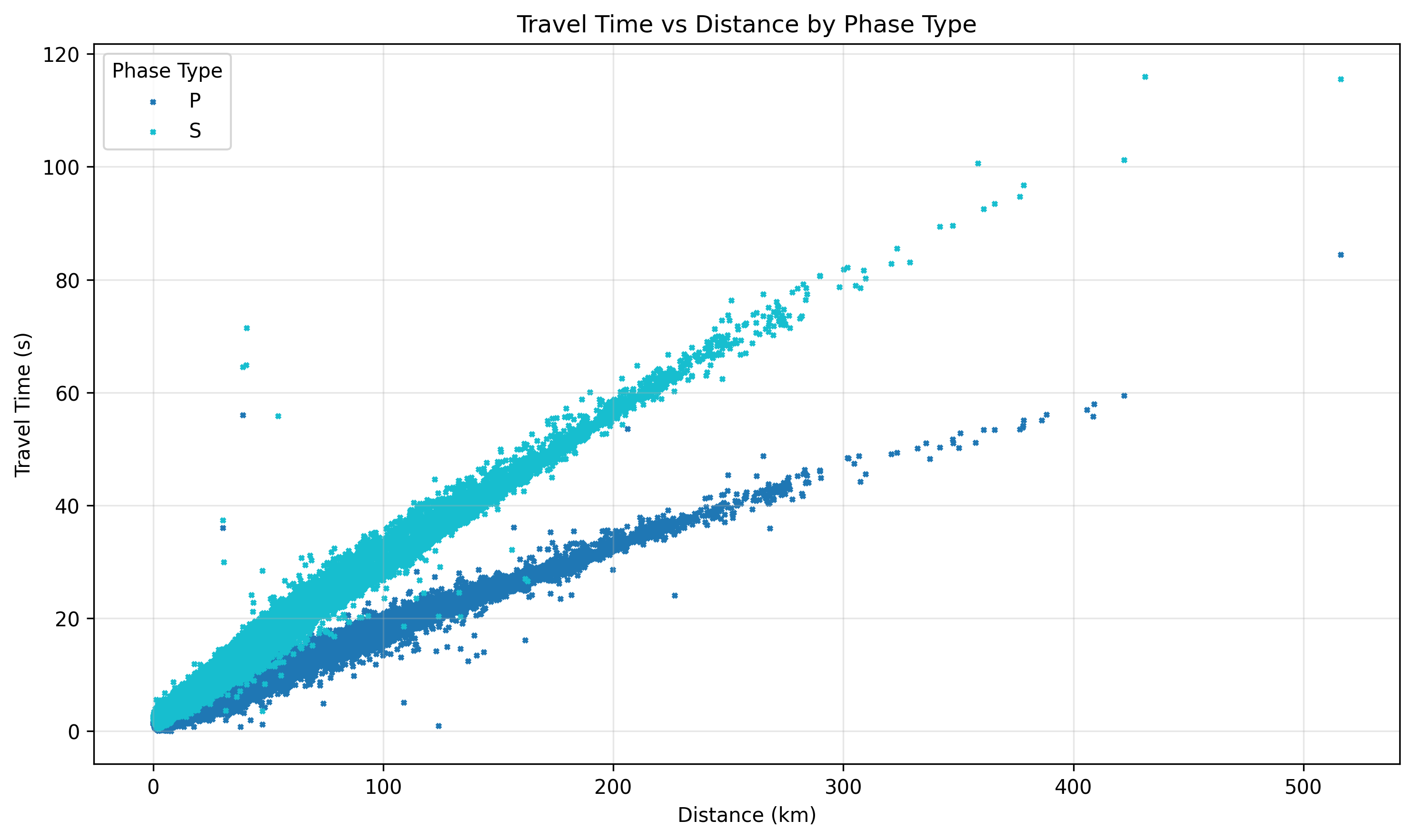
network.plot_travel_time_vs_distance(savepath="travel_time_vs_distance.png")
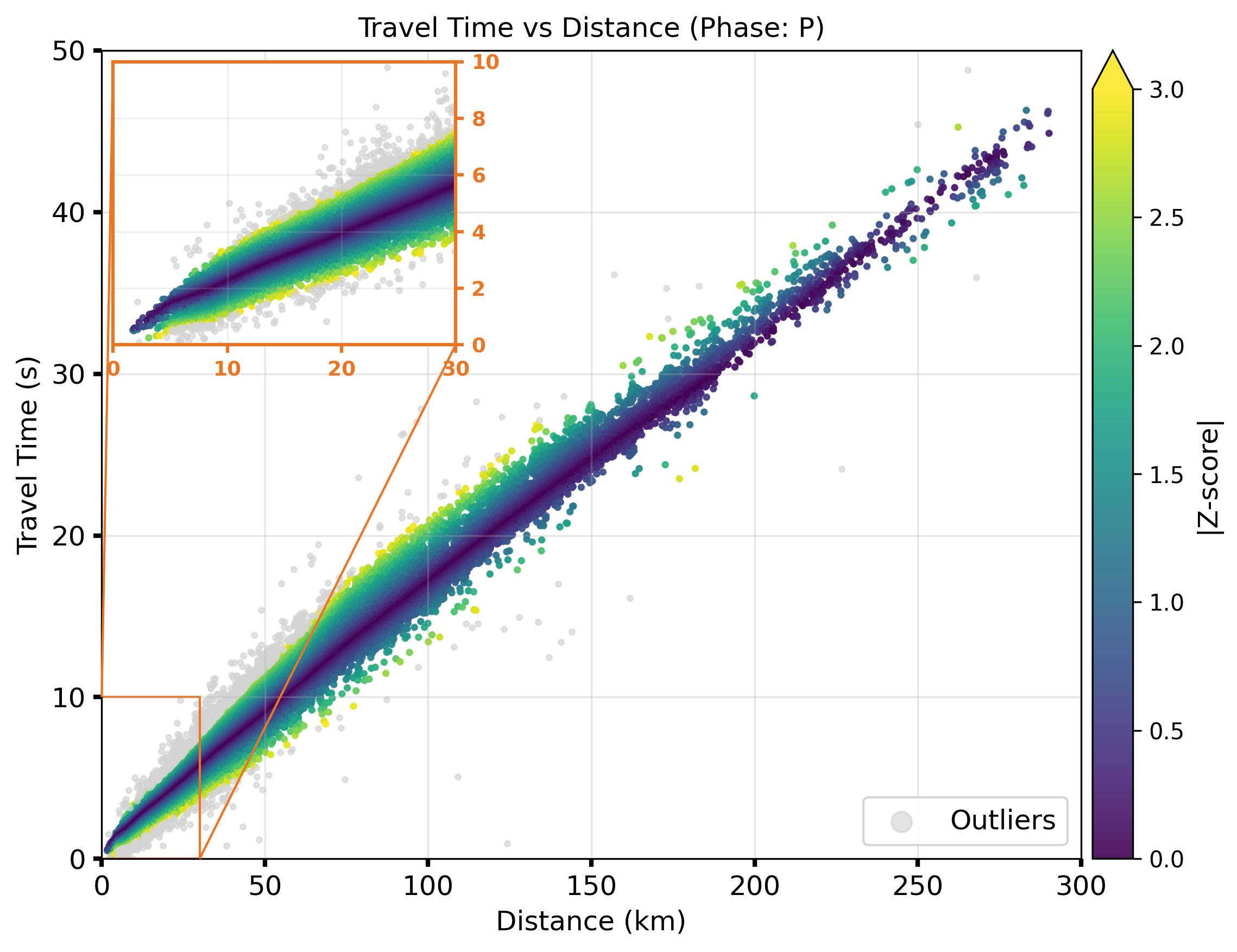
network.plot_travel_time_vs_distance_zscore(savepath="plot_travel_time_vs_distance_zscore.png")

Note

We need Cartopy to be able to plot figures with maps.

Available Figures

The table below summarizes the main categories of figures generated by UTDQuake. These plots are designed to help users quickly evaluate data quality, spatial coverage, and picking performance.

UTDQuake analysis
Overview	Stats	P & S Picks Analysis

Magnitude & Phases Analysis	Uncertainty in station location	Uncertainty in EQ location

General Travel Time Overview	Travel Time	Travel Time Zscore